|
Introduction – an
overview of basic terminology and structure |
Beyond Mapping book |
Coming
to Terms with Terminology — describes
the underlying theory of how point, line and areal features are stored in
Vector and Raster GISs
GIS
Maps Are Dumb — compares
the basic Vector and Raster data structure approaches for storing individual
map layers
Terminology
Accelerates Your Intellectual Depletion Allowance
— introduces
the concepts and organization used in GIS databases comprised of multiple map
layers
<Click here> for a printer-friendly version of this topic
(.pdf).
(Back to the Table of Contents)
______________________________
Coming to Terms with Terminology
(GIS World, July 1993)
…sticks and stones
may break my bones, but terminology will never hurt me
Geographical
Information Systems (GIS) technology has its roots in computer mapping and
spatial data base management. It allows
users to effectively organize, update and query mapped data. More recently, GIS has moved from graphic
inventory of the landscape to modeling potential uses of the land. The evolution from mapping to data management
to modeling is the result of the digital map format and increasing quantification
of map analysis procedures. The new
procedures and resulting decision-making environment require a rethinking of
traditional mapping concepts. Notions of
error propagation, weighted distance measurement, visual exposure surfaces, Nth
optimal path, spatial statistics and fragmentation indices form some of the new
tools confronting the users of GIS.
To
some, the unfamiliar terminology, concepts and capabilities of map analysis
represent the "darker side" of GIS technology. Traditional mapping and data base management
are comfortable turf. You use the
computer to link your file cabinets to your map sheets— it's automation of your
daily routine. Your current concepts are
easily transferred. But the analytic
capabilities of GIS take us well beyond mapping. It challenges old assumptions and suggests
new applications. In many respects, GIS
is more different than it is similar to traditional map processing. The most obvious changes are in the GIS maps
themselves. New terms and concepts
abound. To go beyond mapping, you must
first become comfortable with the basic GIS terminology and organizational
structure. This, and the two sections to
follow, is designed to develop this foundation.
Like
other new technologies, often GIS is guilty of concealing its basic concepts in
unfamiliar terminology. The concepts are
simple; it's the terms that are complicated.
Once you cut through the hyperbole, GIS is a lot like what you do now. In the real world, the landscape is composed
of rocks, dirt, trees and fine feathered friends. In your "paper world," these things
are represented by words, tables and graphics.

Figure
1.
Basic Map Features. Point, lines and areas are stored as
organized sets of coordinates or cells.
Your
maps are graphical abstractions, in which inked lines, shadings and symbols are
used to locate landscape features. Technically speaking, all maps are composed
of three basic features— points,
lines and areas. For example, a typical water map identifies a
spring as a dot, a stream as a squiggle and lake as a blue glob. GIS can reproduce a similar graphic, but that
isn't how it stores the data. In the GIS
world, map features most often are represented by X, Y coordinates, as shown in figure
1. Points are identified as a single
coordinate pair. Lines are identified as
a connected set of points (like "connect-the-dot" pictures). Areas, such as a
ownership parcel, are identified by the coordinates defining their
borders. This comfortable data format is
termed Vector.
A
less familiar format, termed Raster,
uses an imaginary grid of cells to represent the landscape. Points are stored as individual Column, Row entries. Lines are stored as a set of connected
cells. Areas are identified as all of
the cells within the interior of each feature.
Although this data structure has several advantages, it has a major
disadvantage— lack of precision. If a
stream passes through an acre cell, the whole cell is identified as "a
stream." You don't know if it is at
the top, bottom, or wiggles several times through the center of the cell. Further discussion of data structure is best
reserved for later.
For
now, let's see how maps are linked to data.
In the paper world you are the link, running back and forth between a
map and your file cabinets. If you want
to know which timber stands have Douglas fir and Cohassett
soil, you flip through your files and note the stand numbers of those you're
after. You go to the map to locate
them. If you wonder what the forest/soil
type is for a neighboring stand, you run back to the files look it up.
That's
a lot of work for you, but not for your GIS.
The map and file cabinets are electronically linked as shown in figure
2. A common identification number (ID#) is part of the map features and the thematic attribute tables. Actually, these tables are just plain old
data bases— one stores the X, Y's, while the other stores the information about
each stand. Each row of the attribute
table (termed a record)
is divided into several columns termed items).
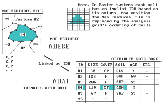
Figure
2.
Linking Features and Attributes.
Tables of map feature location (WHERE) and characteristics (WHAT) are
linked by a common identification number or column, row grid position.
This
organization is similar to the old days when foresters kept data (items) on a
4x5 card (record) for each stand. In
confusing techy-speak, the items COVER= DF and SOIL= COH are searched. In the figure, stand #4 is the only one that
meets the joint condition. Its
coordinates are plotted to the screen and filled with a vibrant color of your
choice. The GIS searches the remaining
40,000 stands and all of the "hits" plotted in less than a
minute. If you "mouse click"
anywhere on the map, the data about that stand pops-up in less than a
second. Think of the shoe leather you
could save.
The
raster world has an analogous link. Each
cell has an implicit ID# based on its column, row position. By convention, the analysis grid is ordered
as you read a book— from left to right, top to bottom. By implication, the first cell (ID# 1) is in
the upper right corner. The next cell
(ID# 2) is the adjacent cell to the right.
The sequential numbering continues through the last column of the first
row. It then picks up with the first
column of the second row, and continues the left to right sequence for each
successive row. It finally finishes with
the lower right cell. Most raster
systems store the "what" information in a separate attribute table
for each map.
Some
systems store the information as one large table with each record indicating a
cell and each item describing a separate thematic attribute. If you think about it (and look at Figure 2)
the similarities between the vector and raster formats should be apparent. The attribute databases are nearly identical
with the exception of the ID#'s— explicit for vector, implicit for raster. The map features file for vector stores
irregular features, whereas for raster, it is an implied analysis grid of
regular cells. There are a lot of
similarities between the two but there are also some significant differences...
as we will soon see.
GIS Maps Are Dumb
(GIS World, August 1993)
When
you view a map, all sorts of things are apparent. If two blue lines come together you instantly
recognize it as a fork in a stream. As
your eye moves along a set of blue lines, you easily comprehend which stream
networks are connected, and which are not.
Your interpretation of the contour lines even tells you which way the
water is flowing.
The
GIS isn't as lucky. With your map view,
you see it all and bring to bear years of experience, insight and
intuition. When a GIS "views"
a map, it does it a piece at a time— you're holistic, it’s myopic. The relationships among the pieces (termed spatial topology) have to be
contained in the data's organization.
The GIS may know that a coordinate pair (X, Y location) is identified
with a stream, but without topology it has no idea how that location relates to
all of the other map locations.
The
fundamental element of map structure is the point, which is represented by a pair of X, Y values. These coordinates usually relate to a
standard referencing grid such as latitude and longitude or UTM meters. There are several types of points, as shown
in Figure 1. Tics are geographic control points used in registering a
map. Discrete points are used to represent information such as
wells. Also, they are used to associate
data with polygons and to the positioning of text. Vertices
and Nodes are used
to construct lines and polygons. This
process is similar to the "connect-the-dots" drawings from your
childhood. You started with the first
dot, and then drew from one to the next until things took shape. Vertices are merely passed through, whereas
nodes identify the special points where more than two lines meet.
The
set of line segments between two nodes is referred to as an Arc. In the case of linear features, such as a
stream network, the GISs keep track of which arcs are connected. Also it notes the up/down stream nodes of
each arc. When the stream flows into a
lake the node is tagged as an inlet. The
stream node at the other end of the lake is identified as an outlet. You see this stuff— the computer has to be
told.
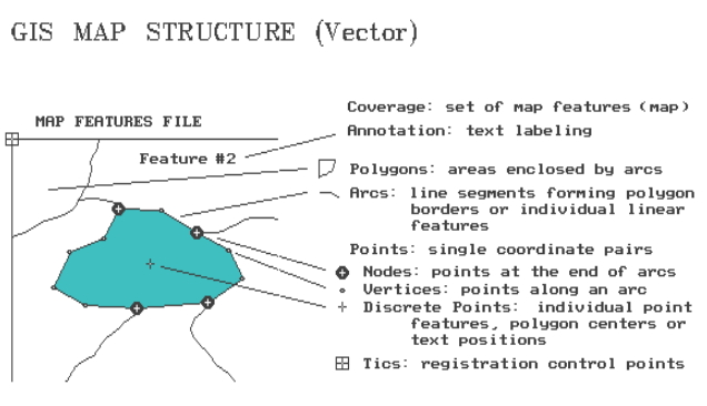
Figure 1. Vector Organization of Map
Features. Map features are formed
by organized sets
of
points (coordinate pairs).
Polygons are areas
enclosed by arcs. Just as several points
form an arc, a closed series of arcs form polygons. There is a discrete point inside each polygon
which serves as a link to the information about it (e.g., size, cover, soil,
age). When polygons are adjoining, such
as timber stands, their shared arcs are tagged with a special code identifying
the linkage. In this manner, the GIS knows the adjoining polygons, and their adjoining polygons,
and so on.
With
minimal guidance from map annotations,
you see all this. However, the GIS must
incorporate it into its data structure.
When it jumps into the middle of a map (termed a Coverage), it has to be
able to sequentially construct all of the relationships among the map
features. Yep, GIS maps are dumb. It's a good thing the computer keeps track of
all the details.
Figure
2 shows the same area expressed in raster format. The entire landscape is covered by an
imaginary grid of cells, the
basic unit of this data structure. There
are two types of cells. A whole cell contains a single map
characteristic throughout its interior (e.g., soil or forest type). A partial
cell contains a mixture of characteristics (e.g., part soils A and
B) or just a portion of an individual characteristic (e.g., road or
spring). It's the partial cells that
account for the lack of precision of raster data. The entire area of a cell is the smallest
addressable unit and all spatial detail smaller than a cell is lost. If a finer analysis grid is used, precision
increases. In theory, the grid could be
as fine as the X, Y coordinates in a vector system,
yielding identical precision. However,
the storage and processing demands at such a high resolution exceed the
capacities of most modern computers.
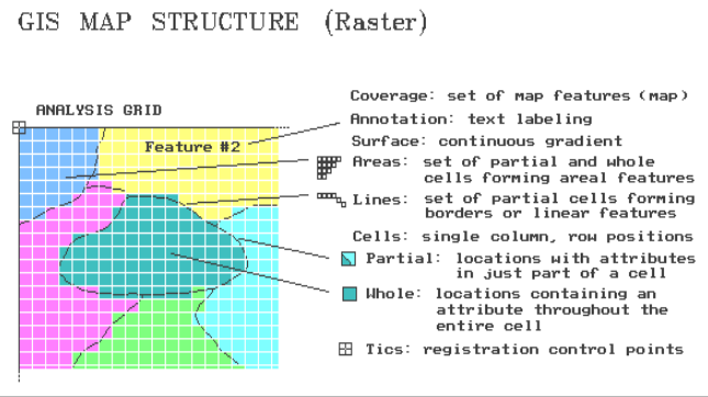
Figure
2.
Raster Organization of Map Features.
All map features are formed by organized sets of cells (column, row in
analysis grid).
Until
there is a super computer on every desk, an oversized partial cell must be used
to identify a single point in space.
Connected series of partial cells are used to identify lines. And, a set of whole (interior) and partial
(border) cells are used to identify areas. To simplify things, the characteristic
dominating a border cell can be assigned, thus making it a whole cell (and a
whole lot easier to store).
The
raster structure allows us to extend the basic map features from just points,
lines and areas, to surfaces. A surface describes the continuous
distribution of gradient data. Elevation
is a good example, at least in hilly terrain.
Each cell is assigned an elevation value that typifies the elevation
within its boundary. The raster format
of elevation data is termed a digital elevation model (DEM) and contains
radically different information than the traditional contour map. Atmospheric pressure, temperature and cost
surfaces are other examples of this new type of map feature. When you think about it, we have just
"scratched the surface" of this strange beast called GIS.
_____________________
Author’s
Note: As with all Beyond Mapping
articles, allow me to apologize in advance for the "poetic license"
invoked in this terse treatment of a complex subject. The specific terms may vary from system to system, however, the basic concepts presented hold for most
systems. For more information see
"Cartographic Data Structures," by Pueker
and Chrisman, American Cartographer, Vol. 2, No. 1, and "Arc/Info: A
Geo-Relational Model for Spatial Information," by S. Morehouse, ESRI, 380
New York Street, Redlands, CA, 92373.
Terminology Accelerates Your Intellectual Depletion Allowance
(GIS World, September 1993)
The
last two sections discussed the basic terminology and approaches in data
structure. However, before we can jump
into the implications of treating maps as data and data structure alternatives,
there is a bigger picture that has to be covered— workspace organization.
Recall that a coverage is the proper term for a
GIS map (vector or raster format alike).
Three things make a GIS coverage different from a traditional map— it's
digital, it represents only one theme and it's seamless. By being
seamless a user can specify a set of corner coordinates and the GIS will
automatically "cut and paste" data from the appropriate storage sections (see Figure 1). This process is similar to you locating four adjoining
topographic sheets, identifying your project area boundary on each, whacking
away with your scissors, and then taping the pieces together. Like sections in the Public Land Survey
System (PLSS), a GIS section is simply a means of dividing a large area into
regular blocks for efficient referencing.
Most users are unaware of the computer's fundamental organization of
sections, as the seamless database structure allows them to define any project
area they please.
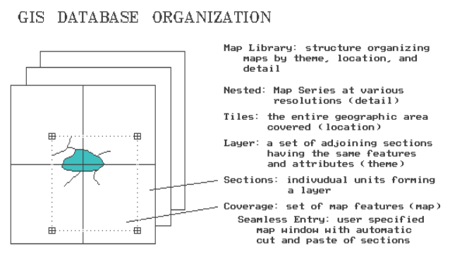
Figure 1. GIS Data Base Organization. In the computer, maps are stored as sets of
adjoining sections.
A
Layer is a set of
adjoining sections having the same features and attributes. For example, a GIS database might contain
separate layers for political jurisdictions, roads, elevation, hydrography, and vegetative cover. In contrast, the familiar USGS topographic
map depicts all these plus other themes on a single map sheet. That's what you see, but that's not really
the case. Actually, each theme is
actually stored as a printer's separate and printed as a sandwich of inked
layers.
It
is imperative that great care is taken in encoding each section or they might
not edge-match. As shown in Figure 1 the boundaries of
features must continue from section to section.
Misalignment of edges is the most frequent cause of pre-mature GIS
death. Obviously, your registration and
digitizing must be extremely precise, but that may not be enough. A couple of uncontrollable problems can
arise. The original maps you're encoding
might not align. If so, adjust them the
best you can. Or, more subversive, the
classification scheme may not be consistent.
For example, you might encode two abutting forest maps with one having
six levels of stocking/age classes, and the other having eight. No matter how carefully you digitize they
will never edge-match (and your GIS is doomed from the start).
A
layer describes the informational content of each GIS map. A Tile
describes the basic geographic area represented in each of the layers. Although tiles are generally rectangular,
they may be any shape, such as a county or forest administration unit. You can think of them as the digital analogue
for the map sheets of a conventional map series.
A
nested map series
contains maps at various resolutions over the same geographic area. This concept is particularly applicable to
raster databases containing different satellite data. Frequently, a user will store two or more
analysis grid resolutions of the same area— a course one for strategic and fine
one for tactical studies. The familiar
USGS's 7.5 and 15 minute topographic series is a "paper product"
example of nesting.
One
final concept ties it all together— the map library. A map
library refers to a listing of all GIS maps in a system. The listing is simultaneously organized by
location, theme and detail. In a
full-featured GIS, you can specify a project area, select the maps you need, then store them in your own workspace. With a healthy understanding of the errors
introduced, you can transform maps of various geographic scales and projections, resample maps of various levels of detail, as
well as exchange vector and raster maps.
|
Data Characterization Column, row entries Features Identification
number Items Map features Points, lines,
areas (polygons) Raster Records Thematic attribute Vector X,Y coordinates Data Organization Edge-match Layers Map Library Nested Seamless Sections Tiles Workspace |
Raster Data Model Area cell set Cell (column, row) Line cell series Partial cell Surfaces Whole cell Vector Data Model Annotation Arcs Coverage Discrete points Nodes Point Polygons Tics Topology Vertices |
Whew! All this has been an overload in both mundane
and arcane terminology. Some of it makes
common sense; some of it may make no sense at all. Keep in mind that you're the intellectual
superior of the GIS. You simply see
things, while it has to organize everything in excruciating detail. Although fundamentally different, you and
your GIS need to be agreeable partners.
The tabular listing above identifies the “terms” of the agreement in the
previous discussions... are you comfortable with them all?
_____________________
Author’s
Note: As with all Beyond Mapping
articles, allow me to apologize in advance for the "poetic license"
invoked in this terse treatment of a complex subject. The specific terms may vary from system to
system; however, the basic concepts presented hold for most systems. For more information see "Cartographic
Data Structures," by Pueker and Chrisman,
American Cartographer, Vol. 2, No. 1, and "Arc/Info: A Geo-Relational
Model for Spatial Information," by S. Morehouse, ESRI, 380 New York Street,
Redlands, CA, 92373.
_______________________________________

(Back to the Table of Contents)