|
Beyond Mapping I Epilog – Historical Overview and What Is in Store |
Beyond
Mapping book |
Bringing the GIS Paradigm to Closure — discusses the evolution and probable
future of GIS technology
Learning Computer-Assisted Map Analysis — a
1986 journal article describing how “old-fashioned math and statistics can go a
long way toward helping us understand GIS”
A Mathematical Structure for Analyzing Maps —
1986 journal article establishing a comprehensive framework for map
analysis/modeling using primitive spatial analysis and spatial statistics
operators
Note: The processing
and figures discussed in this topic were derived using MapCalcTM
software. See www.innovativegis.com
to download a free MapCalc Learner version with tutorial materials for
classroom and self-learning map analysis concepts and procedures.
<Click here> right-click to
download a printer-friendly version of this topic (.pdf).
(Back
to the Table of Contents)
______________________________
Bringing the GIS Paradigm to
Closure
(GIS
World Supplement, July 1992)
Information has always
been the cornerstone of effective decisions.
Spatial information is particularly complex as it requires two
descriptors—Where is What. For thousands of years the link between the
two descriptors has been the traditional, manually drafted map involving pens,
rub-on shading, rulers, planimeters, dot grids, and acetate sheets. Its historical use was for navigation through
unfamiliar terrain and seas, emphasizing the accurate location of physical
features.
More recently, analysis of mapped data has become an important part of
understanding and managing geographic space.
This new perspective marks a turning point in the use of maps from one
emphasizing physical description of geographic space, to one of interpreting
mapped data, combining map layers and finally, to spatially characterizing and
communicating complex spatial relationships.
This movement from “where is what” (descriptive) to "so what and
why" (prescriptive) has set the stage for entirely new geospatial concepts
and tools.
Since the 1960's, the
decision-making process has become increasingly quantitative, and mathematical
models have become commonplace. Prior to
the computerized map, most spatial analyses were severely limited by their
manual processing procedures. The
computer has provided the means for both efficient handling of voluminous data
and effective spatial analysis capabilities.
From this perspective, all geographic information systems are rooted in
the digital nature of the computerized map.
The coining of the term Geographic Information Systems reinforces this movement
from maps as images to mapped data. In
fact, information is GIS's middle name.
Of course, there have been other, more descriptive definitions of the
acronym, such as "Gee It's Stupid," or "Guessing Is
Simpler," or my personal favorite, "Guaranteed Income Stream."
COMPUTER MAPPING
The early 1970's saw computer mapping
automate map drafting. The points, lines and areas defining geographic features
on a map are represented as an organized set of X, Y coordinates. These data
drive pen plotters that can rapidly redraw the connections at a variety of
colors, scales, and projections with the map image, itself, as the focus of the
processing.
The pioneering work during this period established
many of the underlying concepts and procedures of modern GIS technology. An
obvious advantage with computer mapping is the ability to change a portion of a
map and quickly redraft the entire area. Updates to resource maps which could
take weeks, such as a forest fire burn, can be done in a few hours. The less
obvious advantage is the radical change in the format of mapped data— from
analog inked lines on paper, to digital values stored on disk.
SPATIAL DATA MANAGEMENT
During 1980's, the change in data format and
computer environment was exploited. Spatial database management systems
were developed that linked computer mapping capabilities with traditional
database management capabilities. In these
systems, identification numbers are assigned to each geographic feature, such
as a timber harvest unit or ownership parcel.
For example, a user is able to point to any location on a map and
instantly retrieve information about that location. Alternatively, a user can specify a set of
conditions, such as a specific forest and soil combination, then
direct the results of the geographic search to be displayed as a map.
Early in the development of GIS, two alternative
data structures for encoding maps were debated.
The vector data model
closely mimics the manual drafting process by representing map features
(discrete spatial objects) as a set of lines which, in turn, are stores as a
series of X,Y coordinates. An alternative structure, termed the raster data model, establishes an
imaginary grid over a project area, and then stores resource information for
each cell in the grid (continuous map surface).
The early debate attempted to determine the universally best structure. The relative advantages and disadvantages of
both were viewed in a competitive manner that failed to recognize the overall
strengths of a GIS approach encompassing both formats.
By the mid-1980's, the general consensus within the
GIS community was that the nature of the data and the processing desired
determines the appropriate data structure.
This realization of the duality of mapped data structure had significant
impact on geographic information systems.
From one perspective, maps form sharp boundaries that are best
represented as lines. Property
ownership, timber sale boundaries, and road networks are examples where lines
are real and the data are certain. Other
maps, such as soils, site index, and slope are interpretations of terrain
conditions. The placement of lines
identifying these conditions is subject to judgment and broad classification of
continuous spatial distributions. From
this perspective, a sharp boundary implied by a line is artificial and the data
itself is based on probability.
Increasing demands for mapped data focused attention
on data availability, accuracy and standards, as well as data structure
issues. Hardware vendors continued to
improve digitizing equipment, with manual digitizing tablets giving way to
automated scanners at many GIS facilities.
A new industry for map encoding and database design emerged, as well as
a marketplace for the sales of digital map products. Regional, national and international
organizations began addressing the necessary standards for digital maps to
insure compatibility among systems. This
era saw GIS database development move from project costing to equity investment
justification in the development of corporate databases.
MAP ANALYSIS AND MODELING
As GIS continued its evolution, the emphasis turned
from descriptive query to prescriptive analysis of maps. If early GIS users had to repeatedly overlay
several maps on a light-table, an analogous procedure was developed within the
GIS. Similarly, if repeated distance and
bearing calculations were needed, the GIS system was programmed with a
mathematical solution. The result of
this effort was GIS functionality that mimicked the manual procedures in a
user's daily activities. The value of
these systems was the savings gained by automating tedious and repetitive
operations.
By the mid-1980's, the bulk of descriptive query
operations were available in most GIS systems and attention turned to a
comprehensive theory of map analysis.
The dominant feature of this theory is that spatial information is
represented numerically, rather than in analog fashion as inked lines on a
map. These digital maps are frequently
conceptualized as a set of "floating maps" with a common
registration, allowing the computer to "look" down and across the
stack of digital maps. The spatial
relationships of the data can be summarized (database queries) or
mathematically manipulated (analytic processing). Because of the analog nature of traditional
map sheets, manual analytic techniques are limited in their quantitative
processing. Digital representation, on
the other hand, makes a wealth of quantitative (as well as qualitative)
processing possible. The application of
this new theory to mapping was revolutionary and its application takes two
forms—spatial statistics and spatial analysis.
Meteorologists and geophysicists have used spatial statistics for decades to
characterize the geographic distribution, or pattern, of mapped data. The statistics describe the spatial variation
in the data, rather than assuming a typical response is everywhere. For example, field measurements of snow depth
can be made at several plots within a watershed. Traditionally, these data are analyzed for a
single value (the average depth) to characterize an entire watershed. Spatial statistics, on the other hand, uses
both the location and the measurements at sample locations to generate a map of
relative snow depth throughout the watershed.
This numeric-based processing is a direct extension of traditional
non-spatial statistics.
Spatial analysis applications, on the other hand, involve context-based
processing. For example, forester’s can
characterize timber supply by considering the relative skidding and log-hauling
accessibility of harvesting parcels. Wildlife managers can consider such
factors as proximity to roads and relative housing density to map human
activity and incorporate this information into habitat delineation. Land
planners can assess the visual exposure of alternative sites for a facility to
sensitive viewing locations, such as roads and scenic overlooks.
Spatial mathematics has evolved similar to spatial
statistics by extending conventional concepts.
This "map algebra" uses sequential processing of spatial
operators to perform complex map analyses.
It is similar to traditional algebra in which primitive operations
(e.g., add, subtract, exponentiate) are logically sequenced on variables to
form equations. However in map algebra,
entire maps composed of thousands or millions of numbers represent the
variables of the spatial equation.
Most of the traditional mathematical capabilities,
plus an extensive set of advanced map processing operations, are available in
modern GIS packages. You can add,
subtract, multiply, divide, exponentiate, root, log, cosine, differentiate and
even integrate maps. After all, maps in
a GIS are just organized sets of numbers.
However, with map-ematics, the spatial
coincidence and juxtaposition of values among and within maps create new
operations, such as effective distance, optimal path routing, visual exposure
density and landscape diversity, shape and pattern. These new tools and
modeling approach to spatial information combine to extend record-keeping
systems and decision-making models into effective decision support systems.
SPATIAL REASONING AND DIALOG
The future also will build
on the cognitive basis, as well as the databases, of GIS technology. Information systems are at a threshold that
is pushing well beyond mapping, management, modeling, and multimedia to spatial
reasoning and dialogue. In the past,
analytical models have focused on management options that are technically
optimal— the scientific solution. Yet in
reality, there is another set of perspectives that must be considered— the
social solution. It is this final sieve
of management alternatives that most often confounds geographic-based
decisions. It uses elusive measures,
such as human values, attitudes, beliefs, judgment, trust and
understanding. These are not the usual quantitative
measures amenable to computer algorithms and traditional decision-making
models.
The step from technically feasible to socially acceptable is not so much
increased scientific and econometric modeling, as it is communication. Basic to effective communication is
involvement of interested parties throughout the decision process. This new participatory environment has two
main elements— consensus building and conflict resolution.
From this perspective, an individual map is not the objective. It is how maps change as the different
scenarios are tried that becomes information.
"What if avoidance of visual exposure is more important than avoidance
of steep slopes in siting a new electric transmission line? Where does the proposed route change, if at
all?" What if slope is more
important? Answers to these analytical
queries (scenarios) focus attention on the effects of differing perspectives. Often, seemingly divergent philosophical
views result in only slightly different map views. This realization, coupled with active
involvement in the decision process, can lead to group consensus.
However, if consensus is not obtained, mechanisms for resolving conflict come
into play. Conflict Resolution extends the Grateful Dead's
lyrics, "nobody is right, if everybody is wrong," by seeking an
acceptable management action through the melding of different
perspectives. The socially-driven
communication occurs during the decision formulation phase.
It involves the creation
of a "conflicts map" which compares the outcomes from two or more
competing uses. Each map location is
assigned a numeric code describing the actual conflict of various perspectives. For example, a parcel might be identified as
ideal for a wildlife preserve, a campground and a timber harvest. As these alternatives are mutually exclusive,
a single use must be assigned. The
assignment, however, involves a holistic perspective which simultaneously
considers the assignments of all other locations in a project area.
Traditional scientific approaches rarely are effective in addressing the
holistic problem of conflict resolution.
Even if a scientific solution is reached, it often is viewed with
suspicion by less technically-versed decision-makers. Modern resource information systems provide
an alternative approach involving human rationalization and tradeoffs.
This process involves
statements like, "If you let me harvest this parcel, I will let you set
aside that one as a wildlife preserve." The statement is followed by a persuasive
argument and group discussion. The
dialogue is far from a mathematical optimization, but often comes closer to an
acceptable decision. It uses the information
system to focus discussion away from broad philosophical positions, to a
specific project area and its unique distribution of conditions and potential
uses.
CRITICAL ISSUES
The technical hurdles surrounding GIS have been
aggressively tackled over the past four decades. Comprehensive spatial databases are taking
form, GIS applications are accelerating and even office automation packages are
including a "mapping button."
So what is the most pressing issue confronting GIS in the next
millennium?
Calvin, of the Calvin and Hobbes comic strip, puts
it in perspective: "Why waste time learning, when ignorance is
instantaneous?" Why should time be
wasted in GIS training and education?
It's just a tool, isn't it? The
users can figure it out for themselves.
They quickly grasped the operational concepts of the toaster and indoor
plumbing. We have been mapping for
thousands of years and it is second nature.
GIS technology just automated the process and made it easier.
Admittedly, this is a bit of an overstatement, but it does set the stage for
GIS's largest hurdle— educating the masses of potential users on what GIS is
(and isn't) and developing spatial reasoning skills. In many respects, GIS technology is not
mapping as usual. The rights, privileges
and responsibilities of interacting with mapped variables are much more demanding
than interactions with traditional maps and spatial records.
At least as much attention (and ultimately, direct
investment) should go into geospatial application development and training as
is given to hardware, software and database development. Like the automobile and indoor plumbing, GIS
won't be an important technology until it becomes second nature for both
accessing mapped data and translating it into information for decisions. Much more attention needs to be focused
beyond mapping to that of spatial reasoning, the "softer," less
traditional side of geotechnology.
GIS’s development has been more evolutionary, than
revolutionary. It responds to
contemporary needs as much as it responds to technical breakthroughs. Planning and management have always required
information as the cornerstone. Early
information systems relied on physical storage of data and manual
processing. With the advent of the
computer, most of these data and procedures have been automated. As a result, the focus of GIS has expanded
from descriptive inventories to entirely new applications involving
prescriptive analysis. In this
transition, map analysis has become more quantitative. This wealth of new processing capabilities
provides an opportunity to address complex spatial issues in entirely new ways.
It is clear that GIS technology has greatly changed our perspective of a
map. It has moved mapping from a
historical role of provider of input, to an active and vital ingredient in the
"thruput" process of decision-making. Today's professional is challenged to
understand this new environment and formulate innovative applications that meet
the complexity and accelerating needs of the twenty-first century.
______________________
Learning Computer-Assisted Map
Analysis
(GIS
World Supplement, June 1993)
“…old-fashioned math
and statistics can go a long way toward helping us understand GIS”
Geographic
Information Systems (GIS) technology is expanding the computer revolution by integrating
spatial information with the research, planning and management of
forestlands. The teaching of GIS
technology poses problems in the classroom, and innovative ways of learning to
apply the technology are being developed.
Unlike
most other disciplines, GIS technology was born from specialized
applications. A comprehensive theory
tying these applications together is only now emerging. In one sense GIS technology is similar to
conventional map processing, involving traditional maps and drafting aids—pens,
run-on shading, rulers, planimeters, dot grids, and acetate sheets for
light-table overlays. In another sense
these systems provide advanced analytical capabilities, enabling land managers
to address complex issues in entirely new ways.
As
essential as computer-assisted map analysis has become, the technology is
difficult to teach. Practical experience
is required as well as theory, yet very few classrooms can provide extensive
hands-on learning. Most GIS require
expensive and specialized hardware, and even where equipment is available,
instructors are faced with teaching the procedures of a system not designed for
classroom use. Consequently, the
approach most commonly used relies on case studies and selected literature.
Mathematics
provides a useful starting point. In
fact, GIS theory is based on a mathematical framework of primitive map-analysis
operations analogous to those of traditional statistics and algebra. The teacher presents basic data
characteristics and map processing as in a math course. Lectures and exercises provide a general
toolbox for map analysis that embodies fundamental concepts and stimulates
creative application. This toolbox is as
flexible as conventional mathematics in expression relationships among
variables—but with GIS, the variables are entire maps.
The
map analysis toolbox helps resource define and evaluate spatial considerations
in land management. For example, forest
managers can characterize timber supply by considering the relative skidding
and log-hauling accessibility of harvest parcels. Wildlife can consider such factors as
proximity to roads and relative housing density in order to map human activity
and incorporate this information into conventional habitat maps. Forest planners can assess the visual
aesthetics of alternative sites for a facility or clearcut.
The Fundamentals
The
main purpose of a geographic information system is to process spatial
information. The data structure can be
conceptualized as a set of “floating maps” with common registration, allowing
the user to “look” down and across a stack of maps. The spatial relationships of the data can be
summarized (database inquiries) or manipulated (analytic processing). Such systems can be formally characterized as
“internally referenced, automated, spatial information systems …designed for
data mapping, management, and analysis.”
All
GIS contain hardware and software for data input, storage, processing, and
display of computerized maps. The
processing functions of these systems can be grouped into four categories:
computer mapping, spatial database management, spatial statistics, and
cartographic modeling.
Computer
mapping—
Also termed automated cartography, computer mapping
involves the preparation of map products.
The focus of these operations is the input and display of computerized
maps.
Spatial
Database Management— These procedures focus on
the storage component of GIS, efficiently organizing and searching large set of
data for frequency statistics and coincidence among variables. The database allows rapid updating and
examining of mapped information. For
example, a spatial database can be searched for areas of silty-loam
soil, moderate slope, and ponderosa pine forest cover. A summary table or a map of the results can
then be produced.
These
mapping and database capabilities have proven to be the backbone of current GIS
applications. Aside from the significant
advantages of processing speed and ability to handle tremendous volumes of
data, such uses are similar to those of manual techniques. Here is where the parallels to mathematics
and traditional statistics may be drawn.
Because
of those parallels, the generalized GIS structure provides a framework for
discussing the various data types and storage procedures involved in computer
mapping and data management. It also
provides a foundation for advanced analytic operations.
Spatial
statistics—The dominant feature of GIS technology is that spatial
information is represented numerically rather than in an analog fashion, as in
the inked lines of a map. Because of the
analog nature of the map sheets, manual analytic techniques are limited to
nonquantitative processing. Digital
representation, on the other hand, has the potential for quantitative as well
as qualitative processing.
GIS
have stimulated the development of spatial statistics, a discipline that seeks
to characterize the geographic distribution or pattern of mapped data. Spatial statistics differs from traditional statistics
by describing the more refined spatial variation in the data, rather than
producing typical responses assumed to be uniformally distributed in space.
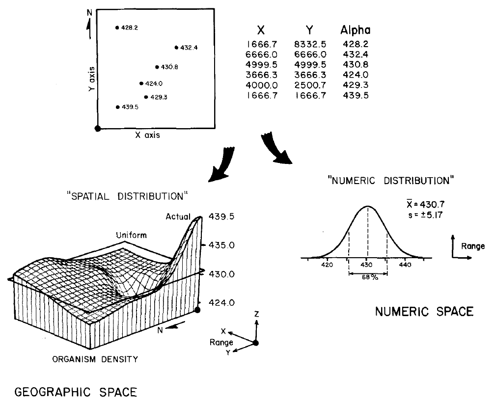
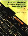
Figure 1. Spatial Statistics.
Whereas traditional statistics identifies the typical response and
assumes this estimate to be uniformally distributed in space, spatial
statistics seeks to characterize the geographic distribution (pattern) of
mapped data. The tabular data identify
the location and population density of microorganisms sampled in a lake. Traditional statistical analysis shows an
average density of about 430, assumed to be uniformally distributed throughout
the lake. Spatial statistics
incorporates locational information in mapping variations in the data. The pattern contains considerable variation
from the average (shown as a plane) in the northwest portion of the lake.
An
example of spatial analysis is shown in figures 1 and 2. Figure 1 depicts density mapping of a
microorganism determined from laboratory analysis of surface water
samples. Figure 2 depicts the natural
extension to multivariate statistics for spatial coincidence between two
microorganisms in the samples.
Traditional
and spatial statistics complement each other for decision-making. In both statistical approaches, the nature of
the data is critical. For analyses
similar to those in Figures 1 and 2, thematic values (“what” information”) must
identify variables that form continuous gradients in both numeric and
geographic space.
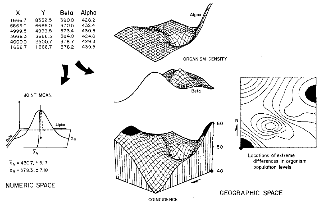
Figure 2. Multivariate Statistics.
Maps characterizing spatial variation among two or more variables can be
compared and locations of unusual coincidence identified. Traditional statistical analysis identifies the
typical paired responses of two microorganism populations. This information assumes that the joint
condition is uniformally distributed in space and does not identify where
atypical joint occurrences might be found.
Spatial statistics compares the two maps of population densities to
identify two areas of unusually large differences in the populations.
Many
forms of mapped data exist, including digital maps which, coupled with
traditional mapping considerations—scale, projection, registration,
resolution—can help foresters understand the potential and pitfalls of GIS
applications. The quantitative nature of
digital maps provides the foundation for a “mathematics
of maps.”
Just
as spatial statistics has been developed by extending concepts of conventional
statistics, a spatial mathematics has evolved.
This “map algebra” uses sequential processing of mathematical primitives
to perform complex map analyses. It is
similar to traditional algebra, in which primitive operations (add, subtract,
exponentiation) are logically sequenced on variables to form equations; but in
map algebra, entire maps composed of thousands of number represent the
variables.
Most
traditional mathematical capabilities plus an extensive set of advanced
map-processing primitives emerge.
Transpose, inverse, and diagonalize are examples of new primitives based
on the nature of matrix algebra. Within
map analysis, the spatial coincidence and juxtapositioning of values among and
within maps create new operators such as masking, proximity, and optimal paths.
This
set of map-analysis operators can be flexibly combined through a processing
structure similar to conventional mathematics.
The logical sequence involves retrieval of one or maps from the
database, processing that data as specified by the user, creation of a new map
containing the processing results, and storage of the new map for subsequent
processing.
The
cyclical processing is similar to “evaluating nested parentheticals” in
traditional algebra. Values for the
“known” variables are first defined, then they are manipulated
by performing the primitive operations in the order prescribed by the
equation.
For
example, in the equation A = (B + C) / D the variables B and C are first
defined and then added, with the sum stored as an intermediate solution. This intermediate value, in turn, is
retrieved and divided by the variable D to derive the value of the unknown
variable A. This same processing
structure provides the framework for computer-assisted map analysis, but the
variables are represented as spatially registered maps. The numbers contained in the solution map (in
effect solving for A) are a function of the input maps and the primitive
operations performed.
Cartographic
modeling—This mathematical structure forms a conceptual framework
easily adapted to a variety of applications in a familiar and intuitive manner.
For example:
(new
value – old value)
%Change =
------------------------------- * 100
old value
This
equation the percent change in value for a parcel of land. In a similar manner, a map of percent change
in land value for an entire town may be expressed in such GIS commands as:
COMPUTE NEWVALUE.MAP MINUS OLDVALUE.MAPFOR
DIFFERENCE.MAP
COMPUTE DIFFERENCE.MAP TIMES 100 DIVIDED BY
OLDVALE.MAP
FOR PERCENTCHANGE.MAP
Within
this model, data for current and past land values are collected and encoded as
computerized maps. These data are
evaluated as shown above to form a solution map of percent change. The simple model might be extended to provide
coincidence statistics, such as
CROSSTAB ZONING.MAPWITH PERCENTCHANGE.MAP
for a table summarizing the spatial
relationship between the zoning map and change in land value. Such a table would show which zones
experienced the greatest increase in market value.
The
basic model might also be extended to include such geographic searches as
RENUMBER PERCENTCHANGE.MAP FOR
BIG_CHANGES.MAP
ASSIGNING 0 TO -20 THRU 20 ASSIGNING 1 TO
20 THRU 100
for a map search that isolates those areas
that experienced more than a +20 percent change in market value.
Analytic Toolbox
In
traditional statistics and mathematics, pencil and paper are all this is needed
to complete exercises. Use of a pocket calculator
or computer enhances this experience by considering larger, more realistic sets
of numbers. However, the tremendous
volume of data involved in even the simplest map-processing task requires a
computer for solution. Also, many of the
advanced operations, such as effective distance measures and optimal paths, are
so analytically complex that computer processing is essential.
Classroom
needs are not being ignored. Software
and materials supporting instruction in computer-assisted map analysis are
appearing on the scene. Among these is
the Map Analysis Package (MAP), a
widely distributed system developed at Yale in 1976 for mainframe
computers. Over 90 universities, many
with natural-resource programs, have acquired these materials.
The
Professional Map Analysis Package (pMAP)
is a commercially developed implementation of MAP for PCs. The Academic
Map Analysis Package (aMAP) is a special
educational version of pMAP available from Yale for classroom use. All of the student exercises can be performed
on a standard IBM PC or similar system.
As
an example of a student exercise, consider the model outlined in figure 3. The exercise proposed that students “generate
a map characterizing both the number of houses and their simple proximity to
major roads, given maps of housing locations (HOUSING) and the road network
(ROADS).” A conceptual flowchart and the
actual sequence of pMAP commands forming the solution
is shown at the top. Some of the
intermediate maps and the final map are shown at the bottom.
Optional
assignments in the exercise required students to “produce a similar map
identifying both the cover type and the distance to the nearest house for all
locations in the study area” and “extend the technique to characterize each map
location as to its general housing density within a tenth-of-a-mile radius, as
well as it proximity to the nearest major road.” Both of these options require minimal
modification of the basic technique—redefinition of the input maps in the first
case and slight editing of two others in the second (see Author’s Note 2 for
more discussion of class exercises and course organization).
GIS
technology is revolutionizing how we handle maps. Beginning in the 1970s, an ever-increasing
portion of mapped data has been collected and processed in digital format. Currently, this computer processing
emphasizes computer mapping and database management. These techniques allow users to update maps
quickly, generate descriptive statistics, make geographic searches for areas of
specified coincidence, and display the results as a variety of colorful and
useful products.
Figure 3. Student Exercise. Proximity to major roads is first determined
and then combined with housing information.
Two-digit codes identify the number of houses (first digit; tens) and
the distance to the nearest major road (second digit; ones).
Emerging
capabilities are extending the revolution to how we analyze spatial
information. These operations provide an
analytic toolbox for expressing spatial relationships within and among maps,
analogous to traditional statistics and algebra. This quantitative approach is changing basic
concepts of map content, structure, and use.
Maps
are moving from images that describe the location of features to mapped data
quantifying a physical or abstract system in prescriptive terms. Students of GIS technology are developing a
proficiency in a sort of “spatial spreadsheet” that allows them to integrate
spatial information with research, planning, and management in natural-resource
fields.
__________________________________
Author’s
Notes: 1) The June
1993 issue of GIS World was a special issue for the URISA conference. This supplemental
white paper is based on a Journal of Forestry paper of the same title
appearing, in the October 1986 issue. 2)
See a 1979 paper entitled “An Academic Approach to Cartographic Modeling
in Management of Natural Resources” describing a graduate-level course in map
analysis/modeling using a “Map Algebra” instructional approach posted at http://www.innovativegis.com/basis/Papers/Other/Harvard1979/HarvardPaper.pdf.
A Mathematical Structure for
Analyzing Maps
(GIS
World Supplement, June 1993)
ABSTRACT—
the growing use of computers in environmental management is profoundly changing
data collection procedures, analytic processes, and even the decision-making
environment itself. The emerging
technology of geographic information systems (GIS) is expanding this revolution
to integrate spatial information fully into research, planning, and management
of land. In one sense, this technology
is similar to conventional map processing involving traditional maps and
drafting aids, such as pens, rub-on shading, rulers, planimeters, dot grids,
and acetate sheets for light-table overlays.
In another sense, these systems provide advanced analytic capabilities,
enabling managers to address complex issues in entirely new ways. This report discusses a fundamental approach
to computer-assisted map analysis that treats entire maps as variables. The set of analytic procedures for processing
mapped data forms a mathematical structure analogous to traditional statistics
and algebra. All of the procedures
discussed are available for personal computer environments.
The
historical use of maps has been for navigation through unfamiliar terrain and
seas. Within this context, preparation
of maps that accurately locate special features became the primary focus of
attention. More recently, analysis of
mapped data has become an important part of resource and environmental
planning. During the 1960s, manual
analytic procedures for overlaying maps were popularized by the work of McHarg (1969) and others.
These techniques mark an important turning point in the use of maps—from
one emphasizing physical descriptors of geographic space, to one spatially
characterizing appropriate land management actions. This movement from descriptive to
prescriptive mapping has set the stage for revolutionary concepts of map
structure, content, and use.
Spatial
analysis involves tremendous volumes of data.
Manual cartographic techniques allow manipulation of these data, but
they are fundamentally limited by their nonquantitative nature. Traditional statistics, on the other hand,
enable quantitative treatment of the data, but, until recently, the sheer
magnitude of mapped data made such processing prohibitive. Recognition of this limitation led to
"stratified sampling" techniques developed in the early part of this
century. These techniques treat spatial
considerations at the onset of analysis by dividing geographic space into
homogeneous response parcels. Most
often, these parcels are manually delineated on an appropriate map, and the
"typical" value for each parcel determined. The results of any analysis
is then assumed to be uniformly distributed throughout each parcel. The area-weighted average of a set of parcels
statistically characterizes the typical response for an extended area. Mathematical modeling of spatial systems has
followed a similar approach of spatially aggregating variation in model
variables. Most ecosystem models, for
example, identify "level variables" and "flow rates"
presumed to be typical for vast geographic expanses.
A
comprehensive spatial statistics and mathematics, for many years, has been variously
conceptualized by both theorist and practitioner. Until modern computers and the computerized
map, these concepts were without practical implementation. The computer has provided the means for both
efficient handling of voluminous data and the quantitative analysis required by
these concepts. From this perspective,
the current revolution in mapping is rooted in the digital nature of the
computerized map. Increasingly, geographic information system (GIS) technology
is being viewed as providing new capabilities for expressing spatial
relationships, as well as efficient mapping and management of spatial
data. This report discusses the
fundamental consideration of the emerging "toolbox" of analytic capabilities.
Geographic
Information Systems (GIS)
The
main purpose of a geographic information system (GIS) is to process spatial
information. These systems can be
defined as internally referenced, automated, spatial information
systems--designed for data mapping, management, and analysis. These systems have an automated linkage
between the type of data, termed the thematic attribute, and the whereabouts of
that data, termed the locational attribute.
This structure can be conceptualized as a stack of "floating
maps," with common spatial registration, allowing the user to
"look" down and across the stack.
The spatial relationships of the data can be examined (that is,
inventory queries) or manipulated (that is, analytic processing). The locational information may be
organized as a collection of line segments
identifying the boundaries of point, linear, and areal features. An alternative organization establishes an
imaginary grid pattern over a study area and stores numbers identifying the
characteristic at each grid space.
Although there are significant practical differences in these data
structures, the primary conceptual difference is that the grid format stores
information on the interior of areal features, and implies boundaries; whereas,
the segment format stores information about boundaries, and implies
interiors. Generally, the line segment
structure is best for inventory-oriented processing, while the grid structure
is best for analysis-oriented processing.
The difficulty of line segments in characterizing spatial gradients,
such as elevation or housing density, coupled with the frequent necessity to
compute interior characteristics limit the use of this data type for many of
the advanced analytic operations. As a
result, most modern GIS contain programs for converting between the two data structures.
Regardless
of the data storage structure, all GIS contain hardware and software for data
input, storage, processing, and display of digital maps. The processing functions of these systems can
be grouped into four broad categories:
-
Computer
mapping
-
Spatial
data base management
-
Spatial
statistics
-
Cartographic
modeling
Most
GIS contain some capabilities from each of these categories. An inventory-oriented system will emphasize
mapping and management functions, whereas, an analysis-oriented system will
focus on statistics and modeling functions.
Computer
mapping, also termed automated cartography, involves the preparation of map
products. The focus of these operations
is on the input and display of computerized maps. Spatial data base management,
on the other hand, focuses on the storage component of GIS technology. Like nonspatial data base systems, these
procedures efficiently organize and search large sets of data for frequency statistics
and/or coincidence among variables. For
example, a spatial data base may be searched to generate a map of areas of silty-loam soil, moderate slope, and ponderosa pine forest
cover. These mapping and data base
capabilities have proven to be the backbone of current GIS applications. Once a data base is compiled, they allow rapid
updating and examining of mapped data. However,
other than the significant advantage of speed, these capabilities are similar
to those of manual techniques. The
remainder of this paper investigates the emerging analytic concepts of spatial
statistics and cartographic modeling.
Spatial
Statistics
Spatial
statistics seeks to characterize the geographic pattern or distribution of
mapped data. This approach differs from
traditional statistics as it describes the spatial variation in the data,
rather than distilling the data for typical responses that are assumed to be
uniformly distributed in space. For example,
consider the hypothetical data presented in Figure 1.
Figure 1. Spatially characterizing data variation. Traditional statistics identifies the typical
response and assumes this estimate to be distributed uniformly in space. Spatial statistics seeks to characterize the
geographic distribution, or pattern, of mapped data.
The
large square at the top is a map of sample locations for a portion of a lake. The tabular data to the right identify both
the location and microorganism density determined from laboratory analysis of
the surface water samples. Traditional statistics
would analyze the data by fitting a numerical distribution to the data to
determine the typical response. Such
density functions as standard normal, binomial, and Poisson could be tried, and
the best-fitting functional form chosen. The lower-right inset characterizes the
fitting of a "standard normal curve" indicating an average organism
density of 430.7 + 5.17 units. These
parameters describing the central tendency of the data in numerical space are assumed
to be uniformly distributed in geographic space. As shown in the lower-left plot, this
assumption implies a horizontal plane at 430.7 units over the entire area. The geographic distribution of the standard deviation
would form two planes (analogous to "error bars") above and below the
average. This traditional approach
concentrates on characterizing the typical thematic response, and disregards
the locational information in the sampled data.
Spatial
statistics, on the other hand, incorporates locational information in mapping
the variation in thematic values. Analogous
to traditional statistics, a density function is fitted to the data. In this
instance, the distribution is characterized in geographic space, rather than
numerical space. To conceptualize this process,
visualize a pillar at each sample location rising above the lake in Figure 1 to
the height of its thematic value (that is, measured organism density). The lower-left inset shows a continuous
surface that responds to the peaks and valleys implied by the pillars of the
sampled data. This surface was fitted by
"inverse-distance-squared weighted averaging" of the sample values using
an inexpensive personal computer software package (Golden 1985). The distribution shows considerable variation
in the data in the southwest portion, tending to conflict with the assumption
that variation is uniformly distributed in space. Analogous to traditional statistics, other
surface fitting techniques, such as Kriging, spline, or polynomial functions,
could be tried and the best-fitting functional form chosen. Analysis of the
residuals, from comparisons of the various surfaces with the measured values,
provides an assessment of fit.
Figure
2 depicts multivariate statistical analysis. If the level of another microorganism was also
determined for each water sample, its joint occurrence with the previously
described organism could be assessed. In
traditional statistics, this involves fitting of a density function in
multivariate statistical space. For the
example, a standard normal surface was fitted, with its “joint mean" and "covariance
matrix" describing the typical paired occurrence. Generally speaking, the second organism occurs
less often (379.3 vs. 430.7) with a negative correlation (-.78) between the two
populations.
The
right portion of Figure 2 depicts an analysis of the spatial distributions of
the two populations. For this analysis
the two maps of population density are compared (that is, one subtracted from
the other) to generate a coincidence surface. A planimetric map of the surface, registered
to the original map of the lake, is on the right side of the figure. The darkened areas locate areas of large
differences (that is, more than average difference plus average standard deviation)
in the two organism populations. The
combined information provided by traditional and spatial statistics complements
each other for decision making. Characterizing
the typical response develops a general impression of the data. The mapping of the variance in the data
refines this impression by locating areas of abnormal response. In the example, the approximately 50 units difference in average population densities may not
warrant overall concern. However, the pockets
of larger differences may direct further investigation, or special management action,
within those areas of the lake.
Figure 2. Assessing coincidence among mapped data. Maps characterizing spatial variation among
two or more variables can be compared and locations of unusual coincidence
identified.
In
both statistical approaches, the nature of the data is crucial. For spatial analyses similar to the example, the
thematic values must be numerically "robust" and the locational
attribute "isopleth." These terms
identify map variables that form gradients in both numeric and geographic
space. By contrast, a variable might
contain "non-robust" values (for instance, arbitrary numbers
associated with soil types) that are discontinuous, or "choropleth,"
in geographic space (for instance, abrupt land use boundaries). A complete discussion of the considerations
dealing with the various types of data in spatial statistics is beyond the introductory
scope of this article. Both Davis (1973)
and Ripley (1981) offer good treatise of this subject.
A
Mathematical Structure for Map Analysis
Just
as a spatial statistics may be identified, a spatial mathematics is also
emerging. This approach uses sequential processing
of mathematical primitives to perform a wide variety of complex map analyses (Berry
1985). By controlling the order in which
the operations are executed, and using a common database to store the
intermediate results, a mathematical-like processing structure is developed. This "map algebra" (Figure 3) is
similar to traditional algebra in which primitive operations, such as addition,
subtraction, and exponentiation, are logically sequenced for specified variables
to form equations; however, in map algebra the variables represent entire maps
consisting of numerous values. Most of
the traditional mathematical capabilities, plus an extensive set of advanced
map processing primitives, comprise this map analysis "toolbox." As with matrix algebra (a mathematics operating
on groups of numbers defining variables), new primitives emerge that are based
on the nature of the data. Matrix algebra's
transposition, inversion, and diagonalization are examples of extended
operations. Within map analysis, the
spatial coincidence and juxtapositioning of values among and within maps create
new operators, such as proximity, spatial coincidence, and optimal paths.
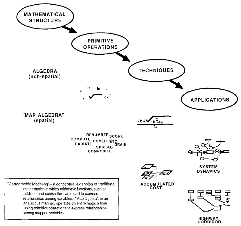
Figure 3. Cartographic modeling. In mathematics, primitive operators, such as
addition and subtraction, are used to express relationships among variables. "Map algebra," in an analogous
manner, operates on entire maps at a time using primitive operators to express
relationships within and among mapped variables.
These
operators can be accessed through general purpose map analysis packages,
similar to the numerous matrix algebra packages. The map analysis package (MAP) (Tomlin 1983)
is an example of a comprehensive general purpose system that has been acquired
by over 350 computer centers throughout the world. A commercial implementation of this system,
the Professional Map Analysis Package (pMAP) (SIS 1986), has recently been
released for personal computers. All of
the processing discussed in this paper was done with this inexpensive pMAP system
in a standard IBM PC environment. The
logical sequencing of map processing involves:
-
Retrieval
of one or more maps from the database
-
Processing
those data as specified by the user
-
Creation
of a new map containing the processing results
-
Storage
of the new map for subsequent processing
Each
new map derived as processing continues is spatially registered to the other
maps in the database. The values
comprising the derived maps are a function of the statistical or mathematical
summary of the values on the "input maps."
This
cyclical processing provides an extremely flexible structure similar to
"evaluating nested parentheticals” in traditional algebra. Within this structure, a mathematician first
defines the values for each dependent variable and then solves the equation by
performing the primitive mathematical operations on those numbers in the order
prescribed by the equation. For example,
the simple equation
A =
(B + C)/D
identifies that the variables B and C are first
defined, and then added, with the sum being stored as an intermediate solution.
The intermediate value, in turn, is divided
by the variable D to calculate the solution variable A. This same mathematical structure provides the framework
for computer-assisted map analysis.
Within
this processing structure, four fundamental classes of map analysis operations
may be identified. These include:
-
Reclassifying maps— involving the
reassignment of the values of an existing map as a function of the initial
value, position, size, shape, or contiguity of the spatial configuration associated
with each category.
-
Overlaying maps— resulting
in
the creation of a new map where the value assigned to every location is computed
as a function of the independent values associated with that location on two or
more existing maps.
-
Measuring distance and connectivity— involving the
creation of a new map expressing the distance and route between locations as
simple Euclidean length, or as a function of absolute or relative barriers.
-
Characterizing and summarizing neighborhoods— resulting
in the creation of a new map based on the consideration of values within the
general vicinity of target locations.
These
major groupings can be further classified as to the basic approaches used by
the various processing algorithms. This
mathematical structure forms a conceptual framework that is easily adapted to
modeling the spatial relationships in both physical and abstract systems. Detailed discussion of the various analytic procedures
is beyond the introductory scope of this article. Reference to the papers by Berry and Tomlin (1982a
and b) provides comprehensive discussion and examples of each of the classes of
operations.
Cartographic
Modeling
The
cyclical processing structure of map analysis enables primitive spatial
operations to be combined to form equations, or "cartographic
models," in a familiar and intuitive manner. For example, in traditional algebra, an
equation for the percent change in value of a parcel of land may be expressed
as
(new
value – old value)
%Change =
------------------------------- * 100
old value
In
a similar manner, a map of percent change in market values for an entire town
may be expressed, in pMAP command language, as:
COMPUTE NEWVALUE.MAP MINUS OLDVALUE.MAP TIMES
100
DIVIDEDBY OLDVALUE.MAP FOR
PERCENTCHANGE.MAP
Within
this model, data for current and past land values are collected and encoded as
computerized maps. These data are
evaluated, as shown above, to form a solution map of percent change. The simple model might be extended to provide
coincidence statistics, such as…
CROSSTABULATE ZONING.MAP WITH PERCENTCHANGE.MAP
…for
a table summarizing the spatial relationship between type of zoning and change
in land value (to answer the question— which zones have experienced the
greatest decline in market value?). The
basic model might also be extended to include geographic searches, such as…
RENUMBER PERCENTCHANGE.MAP ASSIGNING 0 TO --
20 THRU 20
FOR BIGCHANGES.MAP
…for
a map isolating those areas which have experienced more than a + 20% or -20%
change in market value.
Another
simple model is outlined in Figure 4. It
creates a map characterizing the number of houses and their proximity to major
roads, given maps of housing locations (HOUSING) and the road network (ROADS). The model incorporates reclassifying, distance
measuring, and overlaying operations. An
extension to the model (not shown) uses a neighborhood operation to
characterize each map location as to its general housing density within a tenth
of a mile radius, as well as its proximity to roads. Incorporation of this modification requires
the addition of one line of code and slight editing of two others. A working-copy display of the results and
tabular summary is shown at the bottom of Figure 4. The pMAP command sequence for this analysis is
shown in the upper portion.
The
procedure used in the example may be generalized to identify
"type-distance" combinations among any set of features within a
mapped area. Consider the following
generalization:
onemap à X
anothermap à Y
XDIST
= distance as a
fn(x)
z
= (y * 10) + XDIST
compositemap ß Z
Figure 4. A simple cartographic model. This analysis combines the
information on housing locations (HOUSING) and the road network (ROADS) to
derive a map characterizing the number of houses and their proximity to the
nearest major road.
This
"macro" technique may be stored as a command file and accessed at
anytime. For example, the following command
sequence can be entered to assess the covertype (Y) and distance to the nearest
house (x) for all map locations.
Keyboard Entry
ASSOCIATE X WITH HOUSING
ASSOCIATE Y WITH COVERTYPE
READ c:macro.cmd
Stored Command File
SPREAD X TO 9 FOR PROX_X
COMPUTE Y TIMES l0 FOR Y_10
COMPUTE PROX_X PLUS Y_10 FOR Z
DISPLAY Z
Note: the Z map
contains a two-digit code with the “tens digit” indicating the Covertype and
the “ones digit” indicating the proximity to the nearest house. For example a 21 value indicates locations
that are classified as cover type 2 and close to a house (only 1 cell away).
The
ASSOCIATE command temporarily defines specified maps as generalized variables.
The READ command transfers input control to the designated file, and the stored
set of generalized commands are processed as if they were being entered from
the keyboard. When the model is finished
executing, input control is returned to the keyboard for user interactive processing.
Generalized
Structure for Map Analysis
The
development of a generalized analytic structure for map processing is similar
to those of many other nonspatial systems. For example, the popular dBASE
III package contains less than 20 analytic operations, yet they may be flexibly
combined to create "models" for such diverse applications as address lists,
inventory control, and commitment accounting.
Once developed, these logical sequences of dBASE
sentences can be "fixed" into menus for easy end-user operations. A flexible analytic structure provides for
dynamic simulation as well as database management. For example, the Multiplan
"spreadsheet"
package allows users to define the
interrelationships among variables. By
specifying a logical sequence of interrelationships and variables, a financial
model of a company's production process may be established. By changing specific values of the model, the
impact of uncertainty in fiscal assumptions can be simulated. The advent of database management and
spreadsheet packages has revolutionized the handling of nonspatial data.
Computer-assisted
map analysis promises a similar revolution for handling spatial data. For example, a model for siting a new highway
could be developed. The analysis would
likely consider economic and social concerns (for example, proximity to
high housing density, visual exposure to houses), as well as purely engineering
ones (for example, steep slopes, water bodies). The combined expression of both physical and
nonphysical concerns, in a quantified spatial context, is a major benefit. However, the ability to simulate various scenarios
(for instance, steepness is twice as important as visual exposure; proximity to
housing four times as important as all other considerations) provides an
opportunity to fully integrate spatial information into the decision-making
process. By noting how often and where
the optimal route changes as successive runs are made, information on the
unique sensitivity to siting a highway in a particular locale is described.
In
addition to flexibility, there are several other advantages in developing a
generalized analytic structure for map analysis. The systematic rigor of a mathematical approach
forces both theorist and user to consider carefully the nature of the data
being processed, it also provides a comprehensive format for instruction which
is independent of specific disciplines or applications (Berry 1986). In addition, the flowchart of processing succinctly
describes the components of an analysis.
This communication enables decision makers to understand more fully the
analytic process, and actually comment on model weightings, incomplete
considerations, or erroneous assumptions. These comments, in most cases, can be easily
incorporated and new results generated in a timely manner. From a decision-maker's
point of view, traditional manual techniques of map analysis are separate from
the decision itself. They require
considerable time to perform and many of the considerations are subjective in
their evaluation. From this perspective,
the decision maker attempts to interpret results, bounded by the often vague
assumptions and system expression of the technician. Computer-assisted map analysis, on the other
hand, encourages the involvement of the decision maker in the analytic process.
From this perspective, spatial
information becomes an active and integral part of the decision process itself.
Conclusion
Geographic
information system (GIS) technology is revolutionizing how maps are handled. Since the 1970s, an ever-increasing portion of
mapped data is being collected and processed in digital format. Currently, this processing emphasizes
computer mapping and database management capabilities. These techniques allow users to update maps
quickly, generate descriptive statistics, make geographic searches for areas of
specified coincidence, and display the results as a variety of colorful and
useful products. Newly developing capabilities
extend this revolution to how mapped data are analyzed. These techniques provide an analytic
"toolbox" for expressing the spatial interrelationships of maps. Analogous to traditional algebra and
statistics, primitive operations are logically sequenced on variables to form
spatial models; however, the variables are represented as entire maps.
This
quantitative approach to map analysis is changing basic concepts of map
structure, content, and use. From this
perspective, maps move from images describing the location of features to
mapped data quantifying a physical or abstract system in prescriptive terms. This radical change in map analysis has
promoted a more complete integration of spatial information into the
decision-making process.
_______________________
Author’s
Notes: 1) This supplement is based on an article published
in the Journal
of Environmental Management, Springer-Verlag, Vol 11, No. 3, pp.
317-325, 1986. J.K. Berry. 2) The professional map analysis package
(pMAP) described in this article was developed and written by the author and
Dr. Kenneth L. Reed of Spatial Information Systems, Inc. Several of the concepts and algorithms are
based on the widely distributed mainframe map analysis package (MAP) developed
by C. Dana Tomlin (1983) and distributed by Yale University. 3) References:
-
Berry, J. K. 1985. Computer-assisted map analysis:
fundamental techniques. Pages 369-386 in Proceedings of 6th annual
conference, National Computer Graphics Association, Dallas, Texas, April.
-
Berry, J.K. 1986. The academic map analysis package (aMAP) instructions materials. Yale University, School of Forestry
and Environmental Studies, New Haven, Connecticut.
-
Berry, J. K., and C.D. Tomlin. 1982b. Cartographic
modeling: computer-assisted analysis of spatially defined neighborhoods. Pages
227-241 in Conference on energy
resource management, American Planning Association, Vienna, Virginia, October.
-
Davis, J. C. 1973. Statistics and data analysis in
geology. John Wiley and Sons, New York, pp 170-411.
-
Golden Software. 1985. Golden Software Graphics System
Information Manual. Golden Software, Golden, Colorado.
-
McHarg, I. L. 1969.
Design with nature. Doubleday/Natural History Press, Doubleday and Company,
Garden City, New York, 197 pp.
-
Ripley, B. D. 1981. Spatial statistics. Series in
Probability and Mathematical Statistics. John Wiley and Sons, New York, 241 pp.
-
SIS. 1986. The professional map analysis package (pMAP)user's manual and reference. Spatial Information Systems, Omaha,
Nebraska, 228 pp.
-
Tomlin, C.D. 1983. Digital cartographic modeling
techniques in environmental planning. PhD dissertation, Yale University, School
of Forestry and Environmental Studies, New Haven, Connecticut, 298 pp.